Stochastic Process Modeling
Modeling rare-event probabilities and performing hypothesis testing using Binomial, Poisson, and Gaussian distributions. 이항/포아송/가우시안 분포로 희귀 사건 확률을 모델링하고 가설검정을 수행합니다.
Project Overview프로젝트 개요
In quantitative risk management, correctly modeling the probability of rare events (tail risk) is crucial. This project investigates the transition from Binomial distributions to Poisson and Gaussian limits, effectively modeling scenarios like default events or insurance claims.정량 리스크 관리에서는 희귀 사건(테일 리스크) 확률을 정확히 모델링하는 것이 핵심입니다. 이 프로젝트는 이항분포에서 포아송/가우시안 극한으로의 전이를 분석해, 부도 이벤트나 보험 청구 같은 시나리오를 모델링합니다.
The project also applies rigorous statistical hypothesis testing to determine if subpopulations deviate significantly from expected probability distributions, similar to detecting anomalies in market activity.또한 엄밀한 가설검정을 적용해 하위 집단이 기대 분포에서 유의하게 이탈하는지 판단하며, 시장 이상치 탐지와 유사한 문제를 다룹니다.
Key Concepts Implemented구현한 핵심 개념
Poisson Limit Theorem포아송 극한 정리
Modeled low-probability events in large populations, demonstrating how Binomial variances converge to Poisson intensity rates.
Gaussian Approximation가우시안 근사
Applied the Central Limit Theorem to approximate discrete distributions, enabling rapid analytically tractable risk bounds (VaR).
Statistical Hypothesis Testing통계적 가설검정
Calculated Z-scores and p-values to reject null hypotheses, a fundamental skill for backtesting trading strategies against random market noise.
Visual Analysis시각화 분석
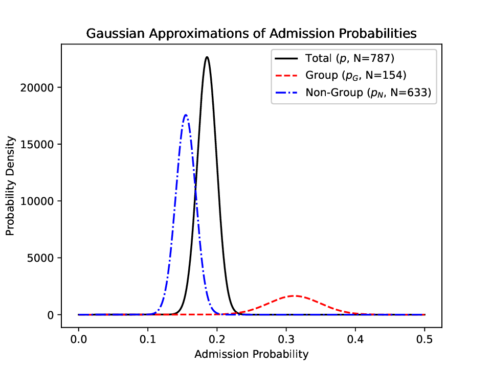
Comparison of probability densities for different population subgroups, illustrating significant statistical deviations (anomalies) detected via Gaussian approximation.
Source Code소스 코드
1. Hypothesis Testing (`p3_hw9.py`)
#!/usr/bin/env python3
import numpy as np
import matplotlib.pyplot as plt
from scipy import stats, special

N_total = 787
N_admit = 146

#Part a
p = N_admit / N_total
sigma_A = np.sqrt(N_total * p * (1 - p))
print(f"a. Standard deviation sigma_A: {sigma_A:.4f}")

#Part b
sigma_p =sigma_A / N_total
print(f"b. Uncertainty in p: {sigma_p:.4f}")

#Part c
N_sub = 154
k_cut = 48
prob_exact = np.sum(stats.binom.pmf(np.arange(k_cut, N_sub + 1), N_sub, p))
print(f"c. Exact probability (k >= 48): {prob_exact:.4e}")

#Part d
mu_sub = N_sub*p
sigma_sub = np.sqrt(N_sub*p*(1-p))
z = (k_cut-mu_sub)/(sigma_sub)
prob_gauss = 0.5*special.erfc(z / np.sqrt(2))
factor = prob_exact/prob_gauss
print(f"d. Gaussian approximation: {prob_gauss:.4e}")
print(f"Factor by Gaussian is small: {factor:.2f}")

#Part e
N_G = 154
N_AG = 48
p_G = N_AG / N_G
sigma_pG = np.sqrt(p_G * (1 - p_G) / N_G)
print(f"e. p_G: {p_G:.4f}, Uncertainty: {sigma_pG:.4f}")

#Part f
N_rem = N_total-N_G
N_Arem = N_admit-N_AG
p_N = N_Arem/N_rem
sigma_pN = np.sqrt(p_N*(1-p_N) / N_rem)
print(f"f. p_N:{p_N:.4f},Uncertainty: {sigma_pN:.4f}")

#Part g
x = np.linspace(0, 0.5, 1000)

def get_y(x, mean, sigma, N):
    return (N / (sigma*np.sqrt(2* np.pi)))*np.exp(-0.5 * ((x - mean) / sigma)**2)

plt.plot(x, get_y(x, p, sigma_p, N_total), color='black', linestyle='solid', label=f'Total ($p$, N={N_total})')

plt.plot(x, get_y(x, p_G, sigma_pG, N_G), color='red', linestyle='dashed', label=f'Group ($p_G$, N={N_G})')

plt.plot(x, get_y(x, p_N, sigma_pN, N_rem), color='blue', linestyle='dashdot', label=f'Non-Group ($p_N$, N={N_rem})')

plt.xlabel('Admission Probability')
plt.ylabel('Probability Density')
plt.title('Gaussian Approximations of Admission Probabilities')
plt.legend()
plt.savefig('p3_hw9.eps')
2. Photon Counting Simulation (`p2_hw9.py`)
#!/usr/bin/env python3
import numpy as np
import matplotlib.pyplot as plt
from scipy.stats import poisson

# Part a
def simulate_photon_count():
    return np.random.binomial(1000, 0.002)

# Part b
counts = [simulate_photon_count() for _ in range(1000)]

# Part c
mu = 1000 * 0.002
x = np.arange(0, np.max(counts) + 3)
y_poisson = 1000 * poisson.pmf(x, mu)

plt.figure()
plt.hist(counts, bins=np.arange(x.max() + 1) - 0.5, rwidth=0.8, label='Simulation')
plt.plot(x, y_poisson, color='red', marker='o', label=f'Poisson ($\mu={mu}$)')
plt.title('Photon Counting Simulation (1000 Trials)')
plt.xlabel('Number of Photons Detected')
plt.ylabel('Frequency')
plt.legend()
plt.savefig('p2_hw9.eps')