Numerical PDE Solver (Finite Difference)

Solving Partial Differential Equations using the Relaxation Method on a discretised 2D grid, applicable to Heat Equations and Black-Scholes models. 이산화된 2D 격자에서 이완법으로 편미분방정식을 풀며, 열방정식과 블랙-숄즈 모델에 적용 가능합니다.

Python Finite Difference Method Numerical Analysis PDEs

Project Overview프로젝트 개요

Partial Differential Equations (PDEs) govern heat diffusion, fluid dynamics, and option pricing in finance (Black-Scholes). This project implements a numerical solver from scratch using the Finite Difference Method to solve Laplace's equation ($\\nabla^2 V = 0$) and other boundary value problems.편미분방정식(PDE)은 열확산, 유체역학, 금융의 옵션 가격결정(블랙-숄즈)을 지배합니다. 이 프로젝트는 유한차분법으로 라플라스 방정식($\\nabla^2 V = 0$) 및 경계값 문제를 푸는 수치해석 솔버를 처음부터 구현합니다.

The implementation uses the "Relaxation Method," an iterative process that converges to the steady-state solution, demonstrating core concepts used in industry-grade PDE solvers for derivative pricing.구현은 반복적으로 정상상태 해에 수렴하는 “이완법”을 사용하며, 파생상품 가격결정에 쓰이는 산업급 PDE 솔버의 핵심 개념을 보여줍니다.

Key Concepts Implemented구현한 핵심 개념

Finite Difference Method유한차분법

Discretized continuous derivatives into difference equations on a grid, converting calculus problems into matrix algebra manageable by computers.

Relaxation Algorithm이완 알고리즘

Implemented an iterative averaging algorithm where each grid point is updated based on its neighbors, simulating the physical process of diffusion.

Boundary Conditions경계 조건

Handled Dirichlet boundary conditions (fixed values at edges) which equate to boundary options or fixed-rate constraints in financial models.

Visual Analysis시각화 분석

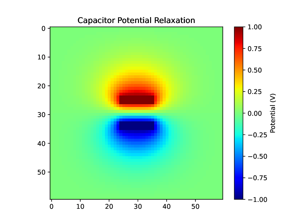
Heatmap visualization of the electric potential field relaxing to a steady state between two capacitor plates. The color gradient represents the potential magnitude.

Source Code: PDE Solver (`p1_hw10.py`)소스 코드: PDE 솔버 (`p1_hw10.py`)

#!/usr/bin/env python3
#First eps file is 256 iterations, gridsize 60, plate thickness 0.05,plate
#width 0.2, gap between plates being 2*plate thickness which is 0.1, and voltage
#equal to 1.
#The second file is 100000 iterations (as I wanted to see if the converging num
#ber changes).
#The last file is the "dipole", as I changed the gap between plates being 10*plate thickness.


import numpy as np
import matplotlib.pyplot as plt
import time

ITER = 256
#ITER=100000
GRIDSIZE = 60
PTH = 0.05
PWID = 0.2
GAP = 2.0 * PTH
#GAP = 10.0 * PTH
VOLTAGE = 1.0

def load_boundary(darray, gridsize):
    """Place predetermined potential at boundary points."""
    clx = int(0.5 * gridsize * (1.0 - PWID))
    cux = gridsize - clx
    capth = (2.0 * PTH + GAP) * gridsize
    cly1 = int(0.5 * (gridsize - capth))
    cuy1 = int(cly1 + gridsize * PTH)
    cly2 = int(cly1 + gridsize * (GAP + PTH))
    cuy2 = gridsize - cly1
    darray[clx:cux, cly1:cuy1] = -VOLTAGE
    darray[clx:cux, cly2:cuy2] = VOLTAGE
    darray[0, :] = 0.0        
    darray[gridsize-1, :] = 0.0 
    darray[:, 0] = 0.0  
    darray[:, gridsize-1] = 0.0

olddata = np.zeros((GRIDSIZE, GRIDSIZE))
newdata = np.zeros((GRIDSIZE, GRIDSIZE))
load_boundary(olddata, GRIDSIZE)

print(f"Starting simulation with {ITER} iterations on grid {GRIDSIZE}x{GRIDSIZE}...")

t0 = time.perf_counter()

for i in range(ITER):
    newdata = 0.25 * (np.roll(olddata, 1, axis=0) + 
                      np.roll(olddata, -1, axis=0) + 
                      np.roll(olddata, 1, axis=1) + 
                      np.roll(olddata, -1, axis=1))
    load_boundary(newdata, GRIDSIZE)
    diff = np.abs(newdata - olddata).sum()
    print('iteration: %d difference sum: %.16f' % (i, diff))
    olddata = np.copy(newdata)

elapsed = time.perf_counter() - t0
print()
print('Time elapsed: %.6f s' % elapsed)

# Plotting
plotarr = np.flipud(olddata.transpose(1, 0))
fig, ax = plt.subplots(dpi=180)
im = ax.imshow(plotarr, interpolation='none', cmap='jet')
plt.colorbar(im, label='Potential (V)')
plt.title("Capacitor Potential Relaxation")
output_filename='capacitor_config_1.eps'
plt.savefig(output_filename,format='eps')
plt.show()

input("\nPress  to exit . . . \n")