Monte Carlo Methods & Stochastic Calculus
Solving deterministic problems through random sampling, with applications in options pricing and risk assessment. 무작위 샘플링으로 결정론적 문제를 푸는 방법을 다루며, 옵션 가격결정과 리스크 평가에 적용합니다.
Project Overview프로젝트 개요
This project explores the power of Monte Carlo simulations to solve complex deterministic problems where analytical solutions are difficult or impossible. By leveraging the Law of Large Numbers, the simulation converges to the true value with an error rate scaling as $1/\\sqrt{N}$. 이 프로젝트는 해석적 해가 어렵거나 불가능한 결정론적 문제를 몬테카를로 시뮬레이션으로 푸는 방법을 탐구합니다. 대수의 법칙에 의해 추정값은 참값으로 수렴하며, 오차는 \(1/\\sqrt{N}\) 스케일로 감소합니다.
In computational modeling, these methods are standard for systems where path-dependency makes closed-form solutions inapplicable. 물리학 연구에서는 경로 의존성 때문에 블랙-숄즈 공식이 적용되지 않는 복잡한 파생상품(아시안/룩백 옵션 등)의 가격결정에 표준적으로 사용됩니다.
Key Concepts Implemented구현한 핵심 개념
Convergence Analysis수렴 분석
Verified the $O(N^{-1/2})$ convergence rate of Monte Carlo integration. This theoretical foundation is critical for estimating computation costs in high-frequency trading simulations.몬테카를로 적분의 \(O(N^{-1/2})\) 수렴률을 검증했습니다. 이는 대규모 시뮬레이션에서 필요한 계산 비용을 추정하는 데 중요합니다.
Stochastic Integration확률적 적분
Implemented numerical integration techniques utilizing random sampling to approximate high-dimensional integrals, a common problem in risk model calibration.무작위 샘플링으로 고차원 적분을 근사하는 수치 적분 기법을 구현했습니다(리스크 모델 캘리브레이션에서 자주 등장).
Variance Reduction분산 감소
Analyzed error metrics to understand stability and precision of the estimates, precursors to implementing variance reduction techniques like Antithetic Variates.추정치의 안정성과 정밀도를 이해하기 위해 오차 지표를 분석했고, 이후 antithetic variates 같은 분산 감소 기법으로 확장할 수 있는 기반을 마련했습니다.
Visual Analysis시각화 분석
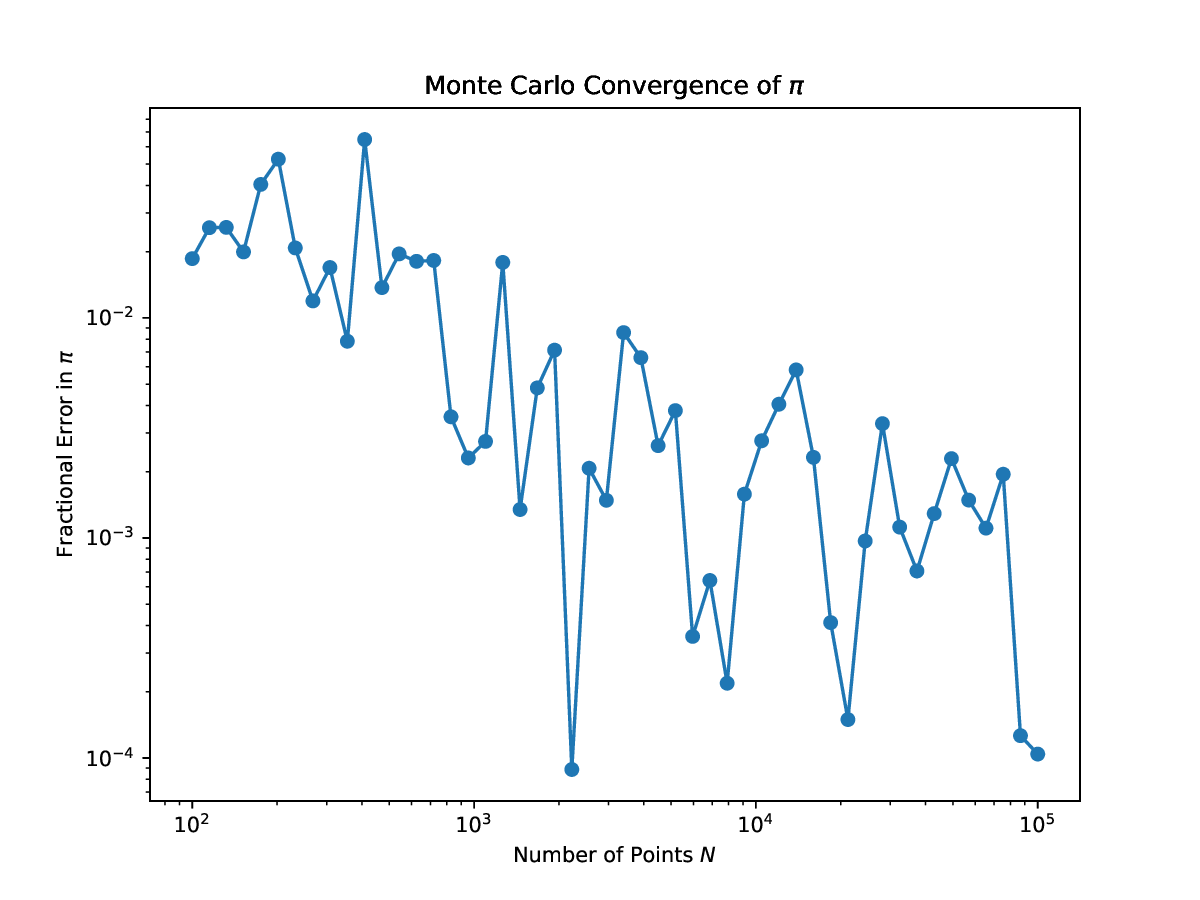
Log-log plot showing the fractional error in estimating $\\pi$ decreasing as the number of samples increases, confirming the $1/\\sqrt{N}$ convergence rate. 샘플 수가 증가할수록 \(\pi\) 추정의 상대 오차가 감소함을 보이는 로그-로그 그래프이며, \(1/\\sqrt{N}\) 수렴률을 확인합니다.
Source Code소스 코드
1. Monte Carlo Integration vs Riemann Sum (`p4_hw9.py`)
#!/usr/bin/env python3
import numpy as np
import matplotlib.pyplot as plt


KNOWN_VALUE = np.sqrt(np.pi)
LIMIT = 10.0

def riemann_sum(N):
    dx = (2 * LIMIT) / N
    x_rect = np.linspace(-LIMIT, LIMIT - dx, N)
    y_rect = np.exp(-x_rect**2)
    return dx * np.sum(y_rect)

def monte_carlo_simulation(N):
    x_mc = np.random.uniform(-LIMIT, LIMIT, N)
    return (2 * LIMIT) * np.mean(np.exp(-x_mc**2))

def main():
    N_values = np.logspace(1, 6, 20, dtype=int)
    rect_errors = []
    mc_errors = []
    for N in N_values:
        #part a
        rect_val = riemann_sum(N)
        r_err = (rect_val - KNOWN_VALUE) / KNOWN_VALUE
        rect_errors.append(abs(r_err))

        #part b
        mc_val = monte_carlo_simulation(N)
        m_err = (mc_val - KNOWN_VALUE) / KNOWN_VALUE
        mc_errors.append(abs(m_err))

    #part a
    plt.loglog(N_values, rect_errors,
               color='blue', linestyle='none', marker='o',
               label='Rectangle Method (Left Sum)')

    plt.xlabel('Number of Rectangles (N)')
    plt.ylabel('Fractional Error (Absolute)')
    plt.title(r'Riemann Sum Error for $\int e^{-x^2} dx$')
    plt.legend()
    plt.savefig('p4_hw9_integration.eps')
    plt.close()

    #part b
    plt.loglog(N_values, mc_errors,
               color='red', linestyle='none', marker='s',
               label='Monte Carlo Simulation')

    plt.xlabel('Number of Random Points (N)')
    plt.ylabel('Fractional Error (Absolute)')
    plt.title(r'Monte Carlo Error for $\int e^{-x^2} dx$')
    plt.legend()
    plt.savefig('p4_hw9_monte_carlo.eps')
    plt.close()

if __name__ == "__main__":
    main()
2. Pi Estimation Convergence (`Monte_Carlo_Convergence_of_pi.py`)
#!/usr/bin/env python3
import numpy as np
import matplotlib.pyplot as plt

N_min=100
N_max=100000

N_values = np.geomspace(N_min, N_max, num=50, dtype=int) #I can also use np.logspace but found out that np.geomspace is better
fractional_errors = []

for N in N_values:
    points = np.random.uniform(0, 2, (N, 2))
    dist_sq = np.sum((points- 1)**2, axis=1)
    pi_est = 4 * np.mean(dist_sq <= 1)
    error = np.abs(pi_est-np.pi) /np.pi
    fractional_errors.append(error)

plt.figure(figsize=(8, 6))
plt.plot(N_values, fractional_errors, 'o-')
plt.xscale('log')
plt.yscale('log')
plt.xlabel('Number of Points $N$')
plt.ylabel('Fractional Error in $\pi$')
plt.title('Monte Carlo Convergence of $\pi$')
plt.savefig('Monte_Carlo_Convergence_of_pi.eps', format='eps')
plt.show()